Going deeper on lesson 9. Every reading you took off the speed trace was one of two operations that have names. This page names them, shows they are the same two operations the lap model runs 729 times, and works both out by hand from the model's own numbers. Nothing new to learn here; only new words for things you did.
Synthetic data. The traces on this page are not measurements. They come from a lap model (our lap model) built from our kart's real numbers - 360 lb, 72/20 gearing, 10.9 in tires, a 6100 rpm limiter, a 0.69 mi track, and the real 58.33 s best lap, which is the only thing the model was tuned to match. The layout is an approximation of Buttonwillow from the track map. When the data logger goes on the kart, the difference between these curves and the real ones becomes the lesson.
1. Slope has a name: the derivative
When you read "how fast is the speed climbing" off the trace, you picked two points and divided the rise by the run. Speed at one time, speed a little later, difference over the time between. That is a derivative: the rate of change of one thing with respect to another.
acceleration = d(speed) / d(time)"d" means "a small change in". Two points from the 72T trace, just after hairpin 2:
at 26.228 s the kart is doing 31.71 mph
at 28.184 s it is doing 37.62 mph
change in speed = 5.91 mph = 8.67 ft/s
change in time  = 1.956 s
acceleration    = 8.67 / 1.956 = 4.43 ft/s^2 = 0.138 g
The model's own long_g column halfway between those points reads 0.137 g. Same number, because the model computed it the same way: two adjacent points, rise over run. The only thing calculus adds is the idea of making the two points closer and closer until the slope is the slope AT a point, not between two. On a 5 ft grid the closest you can get is one step, and that's what the long_g column is.
Every "slope" on lesson 9 was a derivative:
- slope of speed vs time = acceleration (g if you divide by 32.2)
- slope of rpm vs time = how fast the engine is winding up
- slope of the delta-time trace = how fast you are losing (or gaining) time at that point on the track
2. Area has a name: the integral
When you asked "how far did the kart go in those 11 seconds", you added up speed x time over little pieces. That is an integral: the running total of one thing accumulated over another.
distance = integral of speed over timeThe straight, from the model's trace, added up in six coarse pieces (every 44th row, each piece counted as its length x the average of the speeds at its two ends - a "trapezoid"):
six pieces: 863 ft
the model's own 176 pieces: 875 ft
the true straight: 880 ft
More pieces, closer answer. That is the whole content of "taking the limit" in calculus: the answer the sum approaches as the pieces get small. The model uses 5 ft pieces because at 5 ft the error is already below what a logger can resolve (section 4).
Every "area" on lesson 9 was an integral:
- area under speed vs time = distance
- area under acceleration vs time = change in speed
- area under (1/speed) vs distance = time. That last one is the lap model. Lap time = sum over 729 steps of (5 ft / speed there). The model's sum: 58.270 s. Its time column at the last row: 58.272 s.
The two operations undo each other. Slope of the distance curve gives speed back; area under the speed curve gives distance back. That is the fundamental theorem of calculus, and you used both halves of it reading one chart.
3. The delta-time chart is an integral
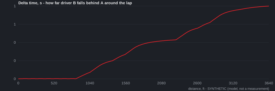
Driver B corners at 1.42 g and brakes at 0.9 g; A at 1.5 and 1.0. The delta trace is B's time minus A's at each point. It is the integral of the time-per-foot difference:
delta(s) = sum over steps of 5 ft x (1/v_B - 1/v_A)(v_A and v_B are the two drivers' speeds at that step, in ft/s, so each term is B's time for the step minus A's.)
Added up over the whole lap that sum is 0.939 s; the model's direct answer is 0.938 s. Read the chart's slope and you get where B loses: flat along the main straight (both on the limiter, no difference to accumulate), steep through every hairpin. One hairpin in numbers: A holds 29.96 mph through the 85 ft arc, B holds 29.15. Time for the arc: A 1.934 s, B 1.988 s. B loses 0.054 s in that one corner, and there are four of them, plus the exits, plus the braking zones. The chart is the running total of all of it, and its final height is the lap-time difference.
Which is the lesson 10 idea, stated properly: the delta trace tells you WHERE time is lost because its slope is the local loss rate, and HOW MUCH because its height is the accumulated loss.
4. Why 5 ft steps are good enough
Every sum on this page is a numerical integral, and its error shrinks with the step. The lap model with its normal 5 ft steps gives 58.270 s. Recomputed skipping every other row (10 ft steps): 58.334 s. Skipping three of four (20 ft): 58.456 s. So halving the step roughly halves the error, and at 5 ft the error is around 0.03 s on a 58 s lap, which is under the 0.05 s a stopwatch thumb can manage and about what a 10 Hz GPS logger (ten position fixes a second) resolves. Going finer than the instrument can see buys nothing.
That is a real design decision in the model, made the calculus way: pick the step where the error is smaller than what you can measure, and stop.
5. What to measure
The data logger samples speed 10 times a second. At 55 mph that is about 8 ft between samples; at 30 mph, about 4.4 ft. Take the real trace, compute acceleration off hairpin 2 from two samples a second apart, the same way as section 1, and compare with 0.138 g. The model thinks the LO206 pulls 0.14 g out of a hairpin. The number the kart actually pulls is the first real derivative of this curriculum, and the difference between the two is lesson 2's torque curve, measured.